Expected value

Expected value runs quietly through finance and machine learning. A trading strategy, a betting system, a learner choosing an action: all of them are judged by what they return on average, over many tries, not by what happened once. This post explains expected value with a settlement example and a lending example, then shows why the average alone is not enough.

It builds on the probability post.

The idea

Plain meaning: if you could live the same risky situation thousands of times, expected value is the average result you would end up with.

How to compute it: list every possible outcome, multiply each one by its probability, and add them up. Bishop and Bishop write it as $\key{E[f]} = \sum_x \risk{p(x)} f(x)$ (equation 2.38); in the notation of this post:

the expected valueprobabilitiesthe cost or loss if it happens

\key{E[X]} = \sum_{i} \bad{x_i} \, \risk{P(x_i)}

Symbol	Meaning
$X$	the uncertain quantity, for example the cost of one trade
$\bad{x_i}$	one possible outcome, for example $2,000
$\risk{P(x_i)}$	the probability of that outcome
$\sum_i$	add up over every possible outcome
$\key{E[X]}$	the expected value of $X$ (read “E of X”)

Example 1: the cost of settling a trade

An operations team looks at last year’s OTC trades. When a trade doesn’t settle on time, it costs money: penalties, funding the gap, staff time. Say the history looks like this:

Outcome	Cost $\bad{x_i}$	Probability $\risk{P(x_i)}$	$\bad{x_i} \times \risk{P(x_i)}$
Settles on time	$0	0.95	$0
One day late	$2,000	0.04	$80
Three or more days late	$15,000	0.01	$150
Total		1.00	$230

\begin{aligned} \key{E[\text{cost}]} &= 0 \times 0.95 \\ &\quad + 2{,}000 \times 0.04 \\ &\quad + 15{,}000 \times 0.01 \\ &= \$230 \end{aligned}

No single trade costs $230. Each one costs $0, $2,000 or $15,000. But on average, each trade costs $230 in fails. With 10,000 trades a month, the team should budget about $2.3 million a month.

Notice the last row. The rare, very late fails are only 1% of trades but make up $150 of the $230. That’s where the money is.

Example 2: expected loss on a loan

Banks use exactly this idea to price credit risk. The expected loss on a loan is usually written as three numbers multiplied together:

\key{\text{EL}} = \risk{\text{PD}} \times \bad{\text{LGD}} \times \bad{\text{EAD}}

Term	Name	Plain meaning
PD	probability of default	the chance the borrower stops paying, usually within a year
LGD	loss given default	the share of the money you lose if they do (after collateral and recovery)
EAD	exposure at default	how much is owed at that moment

A $1,000,000 loan with a 2% chance of default and 45% loss if it defaults:

\key{\text{EL}} = 0.02 \times 0.45 \times 1{,}000{,}000 = \$9{,}000

It’s the same formula as before, just written for one outcome. The loan either defaults (lose $450,000, probability 2%) or it doesn’t (lose $0, probability 98%):

\key{E[\text{loss}]} = 450{,}000 \times 0.02 + 0 \times 0.98 = \$9{,}000

That $9,000 is a cost of doing business. The interest rate has to cover it, plus the bank’s funding cost and a margin, or the loan loses money on average.

Why the average works: many repeats

Expected value only becomes “real” when you repeat the situation many times. This is called the law of large numbers: the more independent repeats, the closer the average result gets to the expected value. Bishop and Bishop’s Deep Learning: Foundations and Concepts writes the same idea as equation 2.40: the plain average of many samples estimates the expected value,

\key{E[f]} \simeq \frac{1}{N} \sum_{n=1}^{N} f(x_n)

and the estimate becomes exact as $N$ grows.

Left: running average loss per loan, jumping around at first and settling near $9,000. Right: distribution of yearly losses for 1,000 loans, centred near $9m but spread from about $5m to over $15m.

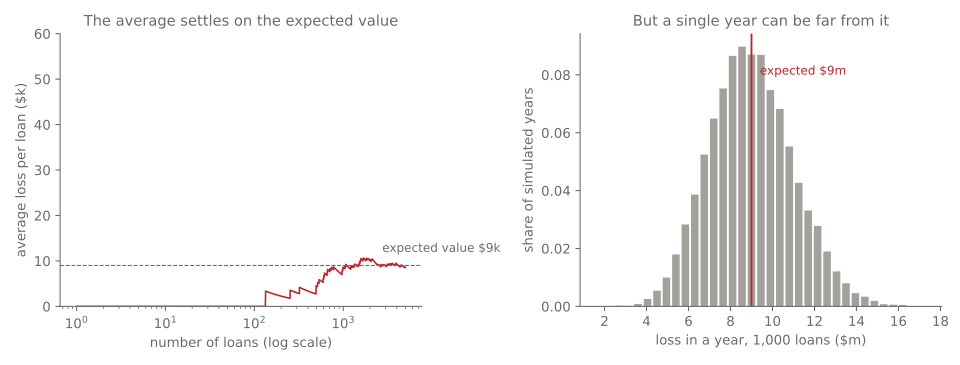
On the left, I simulated loans one by one and tracked the average loss per loan. After 100 loans, the average was still $0: none had defaulted yet. Someone looking only at those 100 loans might think the book was risk-free. After 5,000 loans, the average is $8,550, close to the expected $9,000, and still moving towards it.

Why the average isn’t enough

Now take a book of 1,000 such loans. The expected loss is $1{,}000 \times 9{,}000 = 9{,}000{,}000$ , so $9 million a year. I simulated 20,000 years:

The average yearly loss was $8.99 million, very close to the expected value.
But in 5% of years the loss was more than $12.6 million.
The worst year lost $17.1 million, almost double the average.

That’s the right-hand chart. Expected value tells you the centre. It says nothing about the spread. Two choices can have exactly the same expected value and feel completely different:

Option	Outcomes	Expected value
A	$10,000 for sure	$10,000
B	$0 or $20,000, 50/50	$10,000

Same expected value. Very different risk. Measuring that spread is the job of the standard deviation, which is the next post in this series.

One more honest note: my simulation assumes loans default independently. In real life, defaults cluster. In a recession, many borrowers struggle at the same time. That makes bad years much worse than an independent model suggests. Banks hold capital for exactly this “unexpected” part of the loss, on top of pricing the expected part.

A trader’s example: the biased coin

Romero and Balch’s What Hedge Funds Really Do (chapter 9) uses expected value to explain where a hedge fund’s edge comes from. Bet $1 on a coin flip that you win with probability $p$ : you gain $1 or lose $1, so

\key{E[\text{flip}]} = p \times (+1) + (1 - p) \times (-1) = 2p - 1

A fair coin ( $p = 0.5$ ) is worth nothing on average. A coin with a tiny edge, $p = 0.51$ , is worth 2 cents per dollar per flip. That’s small for one flip, and it’s why skilled traders try to make many independent bets: the expected values add up (the next property) while luck partly cancels out.

A useful property: expected values add up

The expected value of a total is the total of the expected values:

E[X + Y] = \key{E[X]} + \key{E[Y]}

This works even when $X$ and $Y$ are linked, which makes it very handy. The expected loss of a loan book is the sum of the expected losses of its loans. (That’s not true for the risk: for spread, links between loans matter a lot. More on that in the correlation post.)

The code

import numpy as np

# Expected value from a table of outcomes
costs = np.array([0, 2_000, 15_000])
probs = np.array([0.95, 0.04, 0.01])
print((costs * probs).sum())                       # 230.0

# Expected loss on a loan
PD, LGD, EAD = 0.02, 0.45, 1_000_000
print(PD * LGD * EAD)                              # 9000.0

# Simulate 1,000 loans for 20,000 years
rng = np.random.default_rng(1)
defaults = rng.binomial(1_000, PD, 20_000)          # defaults in each year
losses = defaults * LGD * EAD
print(losses.mean(), np.percentile(losses, 95))    # about 9.0m, 12.6m

Summary

Expected value = sum of (outcome × probability). The long-run average.
In credit, EL = PD × LGD × EAD.
It becomes real only over many repeats (law of large numbers).
It says nothing about the spread. Two options with the same expected value can carry very different risk.
Expected values add up, even for linked things. Risk doesn’t.

Mean and standard deviation: how to measure the centre and the spread of real data, like a fund’s daily returns, and why the spread grows with the square root of time.

References

Christopher M. Bishop and Hugh Bishop, Deep Learning: Foundations and Concepts (Springer, 2024), chapter 2, section 2.2: expectation (equation 2.38) and its sample-average estimate (2.40)
Philip J. Romero and Tucker Balch, What Hedge Funds Really Do: An Introduction to Portfolio Management (Business Expert Press, 2014), chapter 9: the expected value of a biased coin
Basel Committee on Banking Supervision, An Explanatory Note on the Basel II IRB Risk Weight Functions (2005), for PD, LGD and EAD as the inputs to credit risk