Bias and variance
ml basics
This is the idea behind overfitting, and it’s explained in section 2.2.2 of An Introduction to Statistical Learning. It’s the reason a model that looks perfect in testing can fail in production, and the reason the next three posts (bagging, random forests, boosting) exist at all.
In the decision trees post, a fully grown tree scored 1.000 on its training trades and 0.584 on new ones. This post explains why, with a formula you can actually measure.
The idea, with a person
Imagine two new settlements analysts predicting how late trades will settle.
- Analyst A has one rule: “late-booked trades are a bit late.” Simple, consistent, and often wrong in the same way. That’s bias: a model too simple for the real pattern.
- Analyst B remembers every single trade they’ve ever seen and predicts from the most similar one. Give B a different month of history, and B’s predictions change completely. That’s variance: a model that reacts too much to the particular data it learned from.
A good analyst is in between: they learn the real pattern and ignore the one-off quirks.
The formula
For a model trained on some data, the expected squared error on a new point splits into three parts. This is equation 2.7 in An Introduction to Statistical Learning:
f̂, the model's predictionf and y, the truthbiasvariance
Written out term by term (same thing, with each part spelled out):
| Symbol | Meaning |
|---|---|
| the true average answer at , the real pattern | |
| what our model predicts at | |
| the model’s average prediction, if we could train it again and again on fresh samples | |
| the variance of the noise: randomness in that no model can predict |
In words:
- Bias²: how far the model’s average guess is from the truth. Too simple → large.
- Variance: how much the model’s guess jumps around depending on the sample it trained on. Too complex → large.
- Noise: the part of the error that stays even with a perfect model.
The expectation here is over many different training samples. That’s the key to understanding variance: it’s not about one model, it’s about how much the model would change if you’d collected different data.
Measuring it
Usually you can’t measure bias and variance, because you don’t know the true pattern . With made-up data, you can. I invented a true curve for how many days late a trade settles, depending on how many hours after the cut-off it was booked, and added random noise with a standard deviation of 0.35 days (so ).
Then, for each tree depth, I repeated this 300 times: draw 80 fresh trades, train a regression tree, record its predictions. That gives me 300 versions of each model, enough to measure its average and its spread.
| Tree depth | Bias² | Variance | Noise | Bias² + variance + noise | Measured error on new trades |
|---|---|---|---|---|---|
| 1 | 0.0226 | 0.0384 | 0.1225 | 0.1836 | 0.1836 |
| 2 | 0.0064 | 0.0249 | 0.1225 | 0.1538 | 0.1540 |
| 3 | 0.0007 | 0.0352 | 0.1225 | 0.1584 | 0.1580 |
| 5 | 0.0002 | 0.0700 | 0.1225 | 0.1927 | 0.1914 |
| 8 | 0.0004 | 0.1080 | 0.1225 | 0.2309 | 0.2308 |
| 15 | 0.0005 | 0.1240 | 0.1225 | 0.2470 | 0.2455 |
Two things to see. First, the formula works: the three parts add up to the error I measured directly on new trades, to within simulation noise. Second, the trade-off:
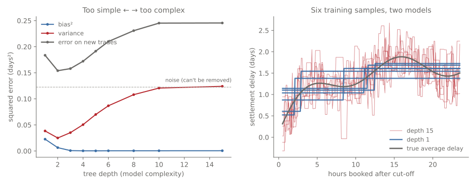
- Depth 1 (blue on the right): a single question. Every version gives nearly the same flat steps, and all of them miss the shape of the curve. High bias.
- Depth 15 (red): every version zig-zags through its own noise, and no two agree. Bias is almost zero, because on average they follow the curve, but each one alone is far off. High variance.
- Depth 2 gives the lowest total error here. Not the most flexible model, not the simplest.
One honest detail: depth 1 has slightly more variance than depth 2. With a single split, the chosen cut-off point jumps around a lot between samples. The general trend (more depth, more variance) holds after that.
Overfitting and underfitting
These are the everyday names:
| Underfitting | Overfitting | |
|---|---|---|
| Cause | Model too simple | Model too complex |
| Main error | Bias | Variance |
| Training error | High | Very low |
| Error on new data | High | High |
| Fix | More flexible model, better features | Simpler model, more data, or averaging |
The tell-tale sign of overfitting is a big gap between training error and error on new data, like the decision tree with a perfect 1.000 on training trades and 0.584 on new ones.
How to find the sweet spot in practice
You never know the true curve in real life, so you can’t compute bias and variance directly. Instead:
- Hold out data. Train on part of the history, test on the rest. Only the test score counts.
- Cross-validation. Split the data into, say, 5 parts. Train on 4, test on the 5th, rotate, and average. More reliable than one split.
- For time series, test forward in time. In finance, never test on dates before your training data. Train on January to June, test on July. Otherwise the model quietly learns from the future.
- Tune complexity on the test score: tree depth, number of features, and so on.
And there’s a third option, which the next posts build on: keep the complex, low-bias model, but reduce its variance by averaging many of them. If each deep tree zig-zags differently, the average of many will follow the real curve. That’s bagging.
The code
import numpy as np
from sklearn.tree import DecisionTreeRegressor
import settlement_data as data           # my helper that generates the made-up delays (not shown)

grid = np.linspace(0.5, 23.5, 200)       # hours late, where we test
truth = data.delay_curve(grid)           # known only because the data is made up

preds = []
for _ in range(300):                     # 300 fresh training samples
    x, y = data.delays(80)
    tree = DecisionTreeRegressor(max_depth=15).fit(x.reshape(-1, 1), y)
    preds.append(tree.predict(grid.reshape(-1, 1)))
preds = np.array(preds)

bias2 = np.mean((preds.mean(axis=0) - truth) ** 2)   # average guess vs truth
variance = np.mean(preds.var(axis=0))                 # how much guesses jump around
Summary
| Idea | Meaning | Remember it as |
|---|---|---|
| Bias | Average guess is off from the truth | Too simple |
| Variance | Guess changes a lot with the training sample | Too sensitive |
| Noise | Randomness in the data itself | Nobody can fix it |
| Decomposition | error = bias² + variance + noise | You can trade one for another |
| Overfitting | training great, new data poor | Too much variance |
| Fixes | simpler model, more data, or average many models | Bagging attacks variance |
Next
Bagging: train many models on slightly different data and average them, cutting variance without adding much bias.
References
- James, Witten, Hastie, Tibshirani and Taylor, An Introduction to Statistical Learning, with Applications in Python (Springer, 2023), section 2.2.2: the bias-variance trade-off (equation 2.7)
- scikit-learn: cross-validation