Linear regression

Linear regression is usually the first model anyone learns, and sections 3.1 to 3.3 of An Introduction to Statistical Learning (ISLP) cover it well. It’s worth learning properly, because it’s simple, fast, easy to explain to a business user, and the starting point for many other models.

This post continues the regression vs classification example: predicting how many OTC trades will fail to settle on a given day.

The idea

You have some days. For each day you know how many trades were booked, and how many failed. Plot them, and they roughly form a line: more trades, more fails. Linear regression finds the one straight line that fits the points best, so you can read off a forecast for any number of trades.

A straight line has two numbers. In the notation of An Introduction to Statistical Learning (ISLP), equations 3.1 and 3.2, with hats marking numbers estimated from data:

β̂ and ŷ, what the model estimatesy, the actual valueRSS and TSS, the error and the spread

\key{\hat{y}} = \key{\hat{\beta}_0} + \key{\hat{\beta}_1} x

Symbol	Meaning	In our example
$x$	the input (feature)	thousand trades booked that day
$\key{\hat{y}}$	the prediction (“y-hat”)	predicted number of fails
$\key{\hat{\beta}_1}$ (“beta-one-hat”)	the slope: how much $\key{\hat{y}}$ goes up when $x$ goes up by 1	extra fails per extra 1,000 trades
$\key{\hat{\beta}_0}$	the intercept: the value of $\key{\hat{y}}$ when $x = 0$	the line’s starting level

What “best” means: least squares

For each day, the line makes a prediction $\key{\hat{y}_i}$ . The real value is $\good{y_i}$ . The difference $\good{y_i} - \key{\hat{y}_i}$ is the residual, the miss.

Linear regression picks the line that makes the residual sum of squares (RSS) as small as possible (ISLP equation 3.3):

\risk{\text{RSS}} = \sum_{i=1}^{n} \left( \good{y_i} - \key{\hat{y}_i} \right)^2

Why square them? Three reasons. A miss above the line and a miss below don’t cancel out. Big misses count much more than small ones. And squaring gives a neat formula for the answer, with no searching needed. This method is called ordinary least squares (OLS).

For one input, the best slope and intercept are (ISLP equation 3.4):

\key{\hat{\beta}_1} = \frac{\sum_i (x_i - \bar{x})(\good{y_i} - \bar{y})}{\sum_i (x_i - \bar{x})^2}

\key{\hat{\beta}_0} = \bar{y} - \key{\hat{\beta}_1} \bar{x}

where $\bar{x}$ and $\bar{y}$ (read “x-bar”, “y-bar”) are the averages.

Plain meaning of the slope formula: the top measures how $x$ and $y$ move together. When a day has more trades than usual, does it also have more fails than usual? The bottom measures how much $x$ moves on its own. Their ratio is “how much $y$ moves per unit of $x$ ”. (The top part, divided by $n-1$ , is the covariance, which gets its own post in this series.)

Worked example: five days by hand

Day	Trades (k) $x$	Fails $y$	$x - \bar{x}$	$y - \bar{y}$	product	$(x - \bar{x})^2$
1	8	70	−4	−25	100	16
2	10	85	−2	−10	20	4
3	12	92	0	−3	0	0
4	14	110	2	15	30	4
5	16	118	4	23	92	16
Average / Sum	$\bar{x} = 12$	$\bar{y} = 95$			242	40

\begin{aligned} \key{\hat{\beta}_1} &= \frac{242}{40} \\ &= 6.05 \end{aligned}

\begin{aligned} \key{\hat{\beta}_0} &= 95 - 6.05 \times 12 \\ &= 22.4 \end{aligned}

\key{\widehat{\text{fails}}} = 22.4 + 6.05 \times \text{trades (k)}

Reading it: each extra 1,000 trades brings about 6 more fails. A day with 13,000 trades: $22.4 + 6.05 \times 13 = 101$ fails expected.

Be careful with the intercept. It says that a day with zero trades has 22.4 fails, which makes no sense. We never saw a day anywhere near zero trades. A line is only trustworthy inside the range of data it learned from. Using it far outside that range is called extrapolation, and it’s how linear models embarrass people.

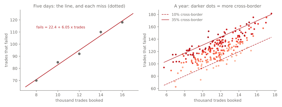
Left: five days with the fitted line and dotted lines showing each miss. Right: a year of days, with two parallel lines for low and high cross-border share.

The dotted lines on the left are the residuals. The fitted line is the one where the squares of those dotted lines add up to the smallest possible total, here 23.9.

How good is the fit? R²

$R^2$ (“R squared”, ISLP equation 3.17) answers: what share of the ups and downs in $y$ does the line explain?

\begin{aligned} R^2 &= 1 - \frac{\risk{\text{RSS}}}{\risk{\text{TSS}}} \\ &= 1 - \frac{\sum_i (\good{y_i} - \key{\hat{y}_i})^2}{\sum_i (\good{y_i} - \bar{y})^2} \end{aligned}

TSS (total sum of squares) is how much $y$ varies around its own average: the error you’d make if you ignored $x$ and always guessed the average.
RSS (residual sum of squares) is the error left over after using the line.

For the five days: TSS $= 25^2 + 10^2 + 3^2 + 15^2 + 23^2 = 1{,}488$ and RSS $= 23.9$ , so

R^2 = 1 - \frac{23.9}{1{,}488} = 0.984

The line explains 98.4% of the day-to-day variation in fails. $R^2 = 0$ means no better than guessing the average. $R^2 = 1$ means perfect.

More than one input

Real days differ in more than trade count. Cross-border trades fail more often, so add the share of cross-border trades as a second input:

\key{\hat{y}} = \key{\hat{\beta}_0} + \key{\hat{\beta}_1} x_1 + \key{\hat{\beta}_2} x_2

Now the “line” is a flat surface in three dimensions, but the idea is the same: find the numbers that make the squared misses smallest.

I made up a year of 250 business days (the hidden rule was 20 + 6 per thousand trades + 150 times the cross-border share, plus random noise). Trained on 187 of them:

	Learned	Hidden rule
Intercept $\key{\hat{\beta}_0}$	13.2	20
Per 1,000 trades $\key{\hat{\beta}_1}$	6.53	6
Per unit of cross-border share $\key{\hat{\beta}_2}$	148.5	150

The model got close to the hidden rule from noisy data alone. Not exact: with noise, the estimates are always a bit off, and they get closer with more data.

Reading $\key{\hat{\beta}_2}$ : a cross-border share 10 percentage points higher (say 30% instead of 20%) means $148.5 \times 0.10 = 14.8$ more fails, with the trade count held the same. That last part matters. In multiple regression, each number is the effect of one input while the others stay fixed.

On the 63 test days the model never saw, $R^2$ was 0.786. With trade count alone it was only 0.383. The second input more than doubled how much of the variation the model explains.

The matrix form (for revision)

With many inputs, the formula is written with matrices. Put the inputs in a matrix $X$ (one row per day, plus a column of 1s for the intercept) and the answers in a vector $y$ . The best coefficients are:

\key{\hat{\beta}} = (X^\top X)^{-1} X^\top y

This comes from the normal equations $X^\top X \key{\hat{\beta}} = X^\top y$ (Murphy, Probabilistic Machine Learning, chapter 11). ISLP doesn’t print the matrix form, because it needs matrix algebra. On the five days it gives exactly $(22.4,\ 6.05)$ , the same as the hand calculation. In practice, libraries solve it with more numerically stable methods than inverting the matrix, but the answer is the same.

The code

import numpy as np
from sklearn.linear_model import LinearRegression

x = np.array([8, 10, 12, 14, 16])          # thousand trades
y = np.array([70, 85, 92, 110, 118])       # fails

# By hand
b1 = ((x - x.mean()) * (y - y.mean())).sum() / ((x - x.mean()) ** 2).sum()
b0 = y.mean() - b1 * x.mean()
print(b0, b1)                               # 22.4  6.05

# With scikit-learn: same answer
model = LinearRegression().fit(x.reshape(-1, 1), y)
print(model.intercept_, model.coef_)        # 22.4  [6.05]
print(model.predict([[13]]))                # [101.]

When linear regression goes wrong

The relationship isn’t a straight line. If fails jump sharply above some volume, a line will miss it. (Decision trees, the next post, handle this.)
Extrapolation. Never trust the line far outside the data, like the “22 fails on a day with no trades”.
Outliers. Because misses are squared, one extreme day (a market outage) can pull the line a long way.
Inputs that move together. If two inputs are strongly linked (trade count and number of counterparties, say), the model can’t tell their effects apart, and the individual numbers become unstable, even when the predictions are fine.
Correlation is not causation. The slope says fails and volume move together. It doesn’t prove one causes the other.

Summary

Idea	Formula	Remember it as
The line	$\key{\hat{y}} = \key{\hat{\beta}_0} + \key{\hat{\beta}_1} x$	Start level plus slope times input
Best fit	minimise $\sum (\good{y_i} - \key{\hat{y}_i})^2$	Least squares
Slope	$\key{\hat{\beta}_1} = \sum (x - \bar{x})(y - \bar{y}) / \sum (x - \bar{x})^2$	How they move together ÷ how $x$ moves alone
Intercept	$\key{\hat{\beta}_0} = \bar{y} - \key{\hat{\beta}_1} \bar{x}$	The line passes through the averages
Fit quality	$R^2 = 1 - \risk{\text{RSS}}/\risk{\text{TSS}}$	Share of the variation explained
Many inputs	$\key{\hat{\beta}} = (X^\top X)^{-1} X^\top y$	The normal equation

Decision trees: a model that asks a series of yes/no questions instead of drawing a line, and can follow patterns a straight line can’t.

References

James, Witten, Hastie, Tibshirani and Taylor, An Introduction to Statistical Learning, with Applications in Python (Springer, 2023), sections 3.1 to 3.3: the model (equations 3.1, 3.2), RSS (3.3), least-squares estimates (3.4), $R^2$ (3.17)
Kevin P. Murphy, Probabilistic Machine Learning: An Introduction (MIT Press, 2022), chapter 11: the normal equations
scikit-learn: ordinary least squares