Mean and standard deviation

Any analysis of returns starts with these two numbers. Almost every measure of a fund or strategy, including the Sharpe ratio, is built from them. The expected value post ended with “two choices can have the same average and very different risk”. This post measures that difference.

First: daily returns

In finance we rarely work with prices directly. We work with returns: the percentage change from one day to the next. This is the definition in Romero and Balch’s What Hedge Funds Really Do (chapter 2):

returns, the datathe meanthe spread: standard deviation, variance

$$\good{r_t} = \frac{p_t}{p_{t-1}} - 1$$

A fund priced $100, then $101: $r = 101/100 - 1 = 0.01 = 1\%$. Returns let you compare a $10 stock with a $1,000 stock on the same scale.

Daily returns compound: to get the return over many days, multiply one plus each day’s return together and subtract one (same chapter):

$$\text{cumulative return} = \prod_{t=1}^{n} (1 + \good{r_t}) - 1$$

Read $\prod$ as “multiply together”, the way $\sum$ means “add together”. That’s why the two funds later in this post end the year at different values despite the same average day.

The mean: where the middle is

Plain meaning: add everything up, divide by how many there are.

$$\key{\bar{r}} = \frac{1}{n} \sum_{t=1}^{n} \good{r_t}$$

Five days of returns: 1%, −2%, 1%, 2%, −1%.

$$\key{\bar{r}} = \frac{1 - 2 + 1 + 2 - 1}{5} = \frac{1}{5} = 0.2\%$$

On an average day, this fund made 0.2%.

The standard deviation: how far things stray

Plain meaning: how far, typically, a day’s return lands from the average.

The recipe:

1. For each day, find how far it is from the mean (the deviation).
2. Square each deviation, so negatives don’t cancel positives.
3. Average the squares. This is the variance.
4. Take the square root, to get back to the original units (percent). This is the standard deviation.

$$\risk{s} = \sqrt{\frac{1}{n-1} \sum_{t=1}^{n} \left( \good{r_t} - \key{\bar{r}} \right)^2}$$

Worked out for the five days (mean 0.2%):

$$\begin{aligned} \risk{s^2} &= \frac{10.8}{5 - 1} \\ &= 2.7 \end{aligned}$$ $$\begin{aligned} \risk{s} &= \sqrt{2.7} \\ &= 1.64\% \end{aligned}$$

A typical day lands about 1.64 percentage points away from the 0.2% average.

Why divide by $n - 1$, not $n$?

This trips everyone up. When you compute the deviations, you measure them from the sample’s own mean, which is pulled towards the data you happen to have. So the deviations come out a little too small on average. Bishop and Bishop’s Deep Learning: Foundations and Concepts shows exactly how much (equation 2.60): the divide-by-$n$ variance comes out, on average, at

$$E\left[\risk{\sigma^2_{\text{ML}}}\right] = \frac{n-1}{n}\,\risk{\sigma^2}$$

of the true variance $\risk{\sigma^2}$. Multiplying by $n/(n-1)$ undoes that, which is the same as dividing by $n - 1$ instead of $n$ (their equation 2.63). It’s called Bessel’s correction, and the result is the sample standard deviation.

Dividing by $n$ gives the population standard deviation, which is right only when you have every possible value, not a sample. Romero and Balch’s What Hedge Funds Really Do (chapter 2) writes volatility with $1/n$; with years of daily data the two versions are practically equal. Here: 1.64% (sample) versus 1.47% (population). With a year of daily data the difference is tiny, but with five days it’s large.

A practical trap: NumPy’s np.std divides by $n$ by default. Pandas’ .std() divides by $n - 1$. Use np.std(x, ddof=1) to get the sample version in NumPy.

Same mean, different risk

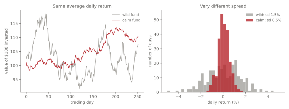
I made up two funds with exactly the same average daily return, 0.04%, but different standard deviations: 0.5% for the calm one, 1.5% for the wild one.

Same average, but the wild fund ended lower. That’s not bad luck. Losses hurt more than equal gains help: lose 10% and then gain 10%, and you’re at 99%, not 100%. The more a fund swings, the more this “volatility drag” eats into growth. A rough rule: the yearly growth rate is about the average return minus half the variance.

From daily to yearly: why √252

There are about 252 trading days in a year. To turn daily numbers into yearly ones, with $\key{\mu}$ for the mean and $\risk{\sigma}$ for the standard deviation:

$$\key{\mu_{\text{annual}}} \approx 252 \times \key{\mu_{\text{daily}}}$$ $$\risk{\sigma_{\text{annual}}} \approx \sqrt{252} \times \risk{\sigma_{\text{daily}}}$$

The mean grows with the number of days, but the standard deviation grows with the square root. Why?

If days are independent, their variances add up. Over 252 days:

$$\risk{\text{Var}}(\text{year}) = 252 \times \risk{\text{Var}}(\text{day})$$ $$\begin{aligned} \risk{\text{SD}}(\text{year}) &= \sqrt{252 \times \risk{\text{Var}}(\text{day})} \\ &= \sqrt{252} \times \risk{\text{SD}}(\text{day}) \end{aligned}$$

Good days and bad days partly cancel out, so risk grows more slowly than time. I checked it by simulating 20,000 years of independent days with a 1% daily standard deviation. The standard deviation of the yearly totals came out at 15.86%. The formula says $\sqrt{252} \times 1\% = 15.87\%$.

For our funds: the calm one is $0.5\% \times \sqrt{252} = 7.94\%$ a year, the wild one 23.81%.

The same $\sqrt{252}$ shows up in the Sharpe ratio, which has its own post later in this series.

The 68–95–99.7 rule, and why markets break it

If returns follow a normal distribution (the bell curve), the standard deviation tells you a lot:

Real market returns are not quite normal. They have fat tails: extreme days happen far more often than the bell curve says. I simulated a million days from a fat-tailed distribution (Student’s t with 3 degrees of freedom) with the same standard deviation:

About 77 times more extreme days (0.62 ÷ 0.008). A risk model that assumes the bell curve will badly underestimate how often a crash day comes. The standard deviation is a good summary of everyday risk, and a poor guide to the worst days.

The code

import numpy as np

returns = np.array([1, -2, 1, 2, -1]) / 100     # five daily returns

mean = returns.mean()                           # 0.002   (0.2%)
sd = returns.std(ddof=1)                        # 0.0164  (1.64%), sample version
sd_pop = returns.std()                          # 0.0147  (1.47%), numpy's default divides by n

# daily to yearly
annual_mean = mean * 252
annual_sd = sd * np.sqrt(252)

# returns from prices
prices = np.array([100, 101, 99, 100, 102, 101])
daily_returns = prices[1:] / prices[:-1] - 1

Summary

Next

Covariance and correlation: how two assets move together, and why combining two risky assets can give you something less risky than either one.

References

• Philip J. Romero and Tucker Balch, What Hedge Funds Really Do: An Introduction to Portfolio Management (Business Expert Press, 2014), chapter 2: returns, cumulative return, volatility
• Christopher M. Bishop and Hugh Bishop, Deep Learning: Foundations and Concepts (Springer, 2024), chapter 2, section 2.3: why dividing by $n$ underestimates variance (equation 2.60) and the $n - 1$ correction (2.63)
• Yves Hilpisch, Python for Finance: Mastering Data-Driven Finance (2nd ed., O’Reilly, 2018), chapter 8, “Financial Time Series”
• NumPy std, for the ddof setting