Covariance, correlation and portfolio variance

Correlation shows up as soon as you look at more than one stock, and it’s at the heart of portfolio construction. The last post measured the risk of one fund. This one answers the question every portfolio manager asks next: what happens to risk when you hold two things together?

Covariance: do two things move together?

Plain meaning: on days when A is above its average, is B also above its average (positive), below it (negative), or neither (around zero)?

how two things move together: ρ and covrisk: σ, s and the covariance matrix Σ

\key{\text{cov}}(A, B) = \frac{1}{n-1} \sum_{t=1}^{n} (a_t - \bar{a})(b_t - \bar{b})

Look at the product $(a_t - \bar{a})(b_t - \bar{b})$ . If both are above average, or both below, the product is positive. If one is up while the other is down, it’s negative. Averaging the products tells you which happens more. (It’s the same $n - 1$ as in the sample standard deviation. In fact, the covariance of a thing with itself is its variance.)

Probability books write the same idea for random variables. Bishop and Bishop’s Deep Learning: Foundations and Concepts (equation 2.48 is the vector version) gives, for two quantities $x$ and $y$ :

\key{\text{cov}}[x, y] = E[xy] - E[x]\,E[y]

“the average of the product, minus the product of the averages”. The sum above is how you estimate it from data.

Worked example: an equity fund and a bond fund

Five made-up days of returns, in percent, chosen to show a strong opposite movement:

Day	Equity fund $a$	Bond fund $b$	$a - \bar{a}$	$b - \bar{b}$	product
1	2	−0.5	1.4	−0.5	−0.70
2	−1	0.5	−1.6	0.5	−0.80
3	3	−1.0	2.4	−1.0	−2.40
4	−2	1.0	−2.6	1.0	−2.60
5	1	0.0	0.4	0.0	0.00
Average / sum	$\bar{a} = 0.6$	$\bar{b} = 0$			−6.5

\key{\text{cov}}(A, B) = \frac{-6.5}{5 - 1} = -1.625

Negative: when equities have a good day, bonds tend to have a bad one, and the other way round.

But what does −1.625 mean? Is that a lot? Covariance is hard to read, because its size depends on the units. Returns in percent give a number 10,000 times bigger than returns as decimals. That’s why we usually use correlation.

Correlation: covariance on a fixed scale

Divide the covariance by both standard deviations:

\key{\rho_{A,B}} = \frac{\key{\text{cov}}(A, B)}{\risk{s_A} \, \risk{s_B}}

The result, $\key{\rho}$ (“rho”), always lies between −1 and +1:

$\key{\rho}$	Meaning
+1	they move perfectly together
0	no straight-line link
−1	they move perfectly opposite

For our funds, $\risk{s_A} = 2.0736$ and $\risk{s_B} = 0.7906$ :

\key{\rho} = \frac{-1.625}{2.0736 \times 0.7906} = -0.991

Almost perfectly opposite. (I made the data that way to make the point clear. In real markets the correlation between stocks and bonds is much weaker, and it changes over time.)

Two warnings:

Correlation only sees straight-line links. Two things can be strongly related in a curved way and still show a correlation near 0.
Correlation is not causation. Two series can move together because a third thing drives both.

Portfolio variance: where correlation pays

Put a share $w_1$ of your money in asset 1 and $w_2 = 1 - w_1$ in asset 2. The portfolio’s variance is (Romero and Balch, What Hedge Funds Really Do, chapter 10):

\risk{\sigma_p^2} = w_1^2 \risk{\sigma_1^2} + w_2^2 \risk{\sigma_2^2} + 2\, w_1 w_2\, \key{\rho}\, \risk{\sigma_1} \risk{\sigma_2}

Symbol	Meaning
$w_1, w_2$	the share of money in each asset (they add to 1)
$\risk{\sigma_1}, \risk{\sigma_2}$	each asset’s standard deviation
$\key{\rho}$	the correlation between them
$\risk{\sigma_p}$	the portfolio’s standard deviation

The first two terms are each asset’s own risk, scaled by how much you hold. The third term is where correlation acts. With $\key{\rho}$ below 1, part of the two risks cancels out. With $\key{\rho}$ negative, the third term is negative and cancels even more.

Worked example: a 60/40 portfolio

Equities with a 20% yearly standard deviation, bonds with 7%, correlation −0.2, held 60/40:

\begin{aligned} \risk{\sigma_p^2} &= 0.6^2 \times 0.20^2 \\ &\quad + 0.4^2 \times 0.07^2 \\ &\quad + 2 \times 0.6 \times 0.4 \times (-0.2) \times 0.20 \times 0.07 \end{aligned}

\begin{aligned} \risk{\sigma_p^2} &= 0.014400 + 0.000784 - 0.001344 \\ &= 0.013840 \end{aligned}

\begin{aligned} \risk{\sigma_p} &= \sqrt{0.013840} \\ &= 11.76\% \end{aligned}

If you just averaged the two risks ( $0.6 \times 20\% + 0.4 \times 7\%$ ), you’d get 14.8%. The real figure is 11.76%. That gap is the diversification benefit. The plain weighted average is only right when the correlation is exactly +1.

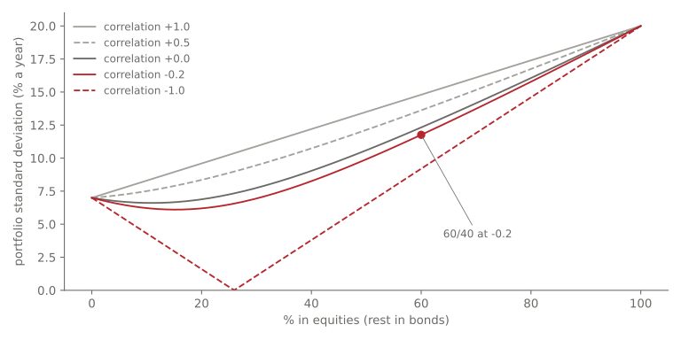
Portfolio standard deviation against the share in equities, one curve per correlation. At +1 it's a straight line; the lower the correlation, the more the curve sags; at −1 it touches zero.

Each curve is one correlation. At +1 (grey, straight), mixing doesn’t reduce risk at all. The lower the correlation, the more the curve sags below the straight line. At −1 (dashed red) it touches zero: a perfect hedge exists.

There’s a mix with the lowest possible risk. For two assets:

w_1^{*} = \frac{\risk{\sigma_2^2} - \key{\rho} \risk{\sigma_1} \risk{\sigma_2}}{\risk{\sigma_1^2} + \risk{\sigma_2^2} - 2 \key{\rho} \risk{\sigma_1} \risk{\sigma_2}}

Here that’s 15.25% in equities, with a standard deviation of 6.10%. That’s lower than holding only bonds (7%), even though you’ve added the riskier asset. Adding something risky made the whole thing safer, because it tends to move the other way.

Many assets: the matrix form

With more than two assets, the same book writes the variance as a sum over every pair of assets:

\risk{\sigma_p^2} = \sum_i \sum_j w_i\, w_j\, \risk{\sigma_i}\, \risk{\sigma_j}\, \key{\rho_{ij}}

where $\key{\rho_{ii}} = 1$ , so each asset’s own variance appears when $i = j$ . The compact way to write it: put the weights in a vector $w$ and all variances and covariances in a covariance matrix $\risk{\Sigma}$ :

\risk{\sigma_p^2} = w^\top \risk{\Sigma}\, w \qquad \risk{\Sigma} = \begin{pmatrix} \risk{\sigma_1^2} & \key{\rho}\,\risk{\sigma_1}\risk{\sigma_2} \\ \key{\rho}\,\risk{\sigma_1}\risk{\sigma_2} & \risk{\sigma_2^2} \end{pmatrix}

The diagonal holds each asset’s variance, and the off-diagonal holds the covariances. For the 60/40 example, $w^\top \risk{\Sigma} w = 0.013840$ , the same as the long formula.

One more useful result. Hold $n$ assets in equal amounts, each with standard deviation $\risk{\sigma}$ and the same correlation $\key{\rho}$ between every pair:

\risk{\sigma_p^2} = \frac{\risk{\sigma^2}}{n} + \left(1 - \frac{1}{n}\right) \key{\rho}\, \risk{\sigma^2}

As $n$ grows, the first term disappears. What’s left is $\key{\rho}\, \risk{\sigma^2}$ , so you can never get the risk below $\sqrt{\key{\rho}}\, \risk{\sigma}$ :

Assets	Correlation 0	Correlation 0.3
1	20.0%	20.0%
10	6.3%	12.2%
100	2.0%	11.1%

With zero correlation, diversification removes almost all the risk. With 0.3, going from 10 assets to 100 barely helps: the floor is $\sqrt{0.3} \times 20\% = 11.0\%$ . That floor is market risk, the part you can’t diversify away.

And the honest catch: correlations are not fixed. In a crisis, many assets fall together and correlations jump up, exactly when you need diversification most.

The code

import numpy as np

a = np.array([2, -1, 3, -2, 1])            # equity fund, daily %
b = np.array([-0.5, 0.5, -1, 1, 0])        # bond fund, daily %
np.cov(a, b)[0, 1]                          # -1.625  (uses n - 1)
np.corrcoef(a, b)[0, 1]                     # -0.991

# 60/40 portfolio risk, two ways
s1, s2, rho, w1, w2 = 0.20, 0.07, -0.2, 0.6, 0.4
var_p = w1**2*s1**2 + w2**2*s2**2 + 2*w1*w2*rho*s1*s2
w = np.array([w1, w2])
Sigma = np.array([[s1**2, rho*s1*s2], [rho*s1*s2, s2**2]])
print(np.sqrt(var_p), np.sqrt(w @ Sigma @ w))    # 0.1176 both

Summary

Idea	Formula	Remember it as
Covariance	$\sum (a_t - \bar{a})(b_t - \bar{b}) / (n-1)$	Do they move together?
Correlation	$\key{\rho} = \key{\text{cov}} / (\risk{s_A} \risk{s_B})$	Covariance on a −1 to +1 scale
Portfolio variance	$w_1^2\risk{\sigma_1^2} + w_2^2\risk{\sigma_2^2} + 2w_1w_2\key{\rho}\risk{\sigma_1}\risk{\sigma_2}$	Correlation decides how much cancels
Matrix form	$w^\top \risk{\Sigma} w$	Same thing, any number of assets
Diversification floor	$\sqrt{\key{\rho}}\,\risk{\sigma}$	Market risk doesn’t diversify away

The Sharpe, Sortino and Information ratios: how to compare two investments that have different returns and different risks.

References

Christopher M. Bishop and Hugh Bishop, Deep Learning: Foundations and Concepts (Springer, 2024), chapter 2: covariance (equation 2.48)
Philip J. Romero and Tucker Balch, What Hedge Funds Really Do: An Introduction to Portfolio Management (Business Expert Press, 2014), chapter 10: portfolio variance, two-asset and general forms
Harry Markowitz, “Portfolio Selection”, The Journal of Finance 7(1), 77–91, 1952
NumPy cov and corrcoef