Random forests

Random forests are covered in section 8.2.2 of An Introduction to Statistical Learning. The method is Leo Breiman’s, from his 2001 paper “Random Forests”. It’s probably the most widely used “just works” model for tabular data in banking: credit scoring, fraud, operations risk.

The bagging post ended on a limit. Averaging many trees cuts variance only down to a floor of $\key{\rho}\,\risk{\sigma^2}$ , where $\key{\rho}$ is how similar the trees’ errors are. Random forests attack $\key{\rho}$ .

The problem with bagging: every tree looks the same

On the made-up settlement data, the strongest single signal of a failed trade is an SSI mismatch (the two banks’ settlement instructions don’t match). I bagged 300 trees and looked at the first question each tree asks:

Model	Trees whose first question is “SSI mismatch?”
Bagging	300 of 300

Each tree sees a different bootstrap sample, but the mismatch signal is so strong that every single tree starts with it, and probably makes similar choices after it. The trees are different, but not very different. Their mistakes are correlated, so averaging them can’t cancel much.

The fix: limit the choice at each split

A random forest adds one rule to bagging:

At every split, pick a random subset of $\key{m}$ features, and only consider those.

Sometimes “SSI mismatch” isn’t in the subset. Then the tree has to find the next-best question using the other features, and it learns something the other trees didn’t.

Model	Features allowed per split	Trees starting with “SSI mismatch?”
Bagging	all 5	300 of 300
Random forest	2 of 5	122 of 300
Random forest	1 of 5	70 of 300

Now the trees genuinely differ: some start with how late the trade was booked, some with the new counterparty, some with cross-border. Each is a bit weaker on its own, but they are wrong in more different ways, so their average is better.

How big should $\key{m}$ be? With $p$ features, the usual starting point is

m, the features each split may use; ρ, how alike the trees arevariance

\key{m} \approx \sqrt{p}

which is what ISLP recommends and what scikit-learn’s RandomForestClassifier uses by default. For regression, The Elements of Statistical Learning suggests $\key{m} \approx p/3$ , but note that scikit-learn’s RandomForestRegressor defaults to all features, which is plain bagging, so set it yourself. These are starting points, not laws: tune $\key{m}$ on held-out data. Setting $\key{m} = p$ turns a random forest back into plain bagging.

The results

Same 15,000 training trades and 5,000 test trades as in the earlier posts. Every tree is grown until its leaves hold 20 trades, so the only difference between rows is the randomness. Scores are AUC on the test trades (0.5 is a coin flip, 1.0 is perfect):

Model	Test AUC
One tree	0.747
Bagging, 300 trees	0.782
Random forest, 300 trees, 2 of 5 features per split	0.795
Random forest, 300 trees, 1 of 5 features per split	0.799
Extra trees, 300 trees, 2 of 5 features, random cut-offs	0.812

Each step adds more randomness, and each step helps. The last row is a variation called extremely randomised trees (scikit-learn’s ExtraTreesClassifier). It also picks the cut-off values at random instead of searching for the best one, which makes the trees even more different and very fast to train.

With only five features, the gains are modest. Random forests shine most with many features, where a few strong ones would otherwise dominate every tree.

Which features matter?

Random forests can report how much each feature contributes. There are two common ways, and they can disagree badly.

Impurity importance (scikit-learn’s feature_importances_): add up how much each feature reduced Gini impurity across all the splits in all the trees. It’s free, since it comes from training.

Permutation importance: take the test set, randomly shuffle one feature’s column so it no longer carries any information, and measure how much the test score drops. The bigger the drop, the more the model relied on that feature.

Feature	Impurity importance	Permutation importance (drop in test AUC)
SSI mismatch	0.520	0.158
Hours booked late	0.204	0.065
Trade size	0.179	0.000
New counterparty	0.050	0.026
Cross-border	0.047	0.036

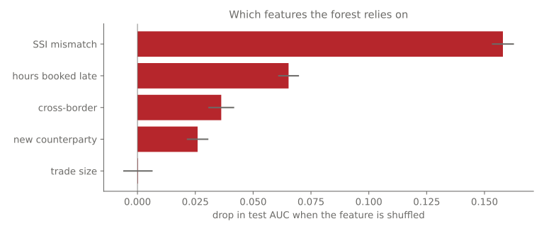
Bar chart of permutation importance: SSI mismatch far ahead, then hours booked late, cross-border, new counterparty; trade size zero.

Look at trade size. Impurity importance ranks it third. Permutation importance says shuffling it costs nothing. In my made-up data, trade size has only a tiny real effect on fails, so the second answer is the honest one.

Why does impurity importance get it wrong? Trade size is a continuous number with thousands of different values, so it offers thousands of possible cut-offs. With that many tries, some cut-off always reduces impurity a little on the training data, by fitting noise. Features like that get inflated scores. scikit-learn’s own documentation warns about exactly this bias towards features with many unique values. For anything you’ll act on, use permutation importance on test data.

The code

from sklearn.ensemble import RandomForestClassifier
from sklearn.inspection import permutation_importance

forest = RandomForestClassifier(
    n_estimators=300,          # number of trees
    max_features=2,            # features considered at each split (m)
    min_samples_leaf=20,       # stop splitting below 20 trades
    n_jobs=-1,                 # use all CPU cores
    random_state=0,
)
forest.fit(X_train, y_train)
forest.predict_proba(X_test)[:, 1]                     # probability of a fail

result = permutation_importance(forest, X_test, y_test, scoring="roc_auc", n_repeats=10)
result.importances_mean                                # drop in AUC per shuffled feature

Why banks like random forests

Few settings to get wrong. The defaults are usually decent.
Hard to overfit by adding trees. More trees never makes it worse; it just stops improving.
Handles mixed data (yes/no flags, amounts, counts) without scaling.
Built-in honesty check: out-of-bag scores, as in bagging.

And the trade-offs: a forest of 300 trees is much harder to explain to a regulator or a business user than one tree, and it’s slower to score. Model risk teams usually ask for importance analysis and example explanations alongside it.

Summary

Idea	Rule	Remember it as
Random forest	bagging + random subset of $\key{m}$ features at each split	force the trees to differ
Why it works	lower correlation $\key{\rho}$ between trees	lower floor $\key{\rho}\risk{\sigma^2}$ on variance
Default $\key{m}$	$\sqrt{p}$ (set it yourself for regression in scikit-learn)	then tune it
Extra trees	also random cut-offs	even more different, very fast
Importance	prefer permutation importance on test data	impurity importance favours many-valued features

Boosting: instead of training trees independently and averaging, train them one after another, each one focusing on the mistakes of the ones before.

References

James, Witten, Hastie, Tibshirani and Taylor, An Introduction to Statistical Learning, with Applications in Python (Springer, 2023), section 8.2.2
Kevin P. Murphy, Probabilistic Machine Learning: An Introduction (MIT Press, 2022), chapter 18: random forests
Hastie, Tibshirani and Friedman, The Elements of Statistical Learning (2nd ed., Springer, 2009), chapter 15
Leo Breiman, “Random Forests”, Machine Learning 45(1), 5–32, 2001
Pierre Geurts, Damien Ernst and Louis Wehenkel, “Extremely randomized trees”, Machine Learning 63(1), 3–42, 2006
scikit-learn: permutation importance vs impurity-based importance