Bagging
ml basics
Bagging is covered in section 8.2 of An Introduction to Statistical Learning. The method comes from Leo Breiman’s 1996 paper “Bagging Predictors”. The name is short for bootstrap aggregating.
The bias and variance post ended with a problem: a deep tree has almost no bias but huge variance. Its answer depends heavily on which data it happened to see. Bagging fixes that by averaging many trees.
The idea: ask a committee
If you ask one settlements analyst how late a trade will settle, you get their answer, quirks and all. Ask twenty analysts who each learned from a slightly different set of past trades, and take the average: their individual quirks partly cancel out, and what’s left is closer to the real pattern.
Bagging does this with models:
- Make many bootstrap samples of the training data.
- Train one model (usually a deep decision tree) on each.
- Average their predictions. For classification, average their probabilities, or take a vote.
Step 1: the bootstrap sample
A bootstrap sample is drawn from the training data with replacement, and it has the same size as the original. Some rows get picked more than once, some not at all.
Eight trades, numbered 1 to 8, and three bootstrap samples of them:
| Sample | Rows drawn | Left out |
|---|---|---|
| 1 | 1, 3, 7, 7, 7, 7, 8, 8 | 2, 4, 5, 6 |
| 2 | 1, 1, 2, 5, 5, 7, 7, 8 | 3, 4, 6 |
| 3 | 2, 3, 4, 7, 7, 7, 8, 8 | 1, 5, 6 |
Each tree sees a different version of the history, so each tree comes out different.
How many rows does a bootstrap sample leave out? The chance that a given row is not picked in one draw is . Over draws:
ρ, how alike the trees' errors arevariance
So each tree never sees about 37% of the data. With 10,000 rows, I measured 36.7%. Those left-out rows are called out-of-bag rows, and they’re useful: each tree can be tested on the rows it never saw, which gives a free estimate of performance without a separate test set.
Step 3: why averaging reduces variance
An Introduction to Statistical Learning (section 8.2.1) starts from a simple fact: averaging independent numbers, each with variance , gives an average with variance . Bagged trees aren’t independent, though: they learn from overlapping data. If you average predictions that each have variance , and every pair has correlation , the average has variance (The Elements of Statistical Learning, equation 15.1):
| Symbol | Meaning |
|---|---|
| number of models averaged | |
| variance of one model’s prediction | |
| correlation between two models’ predictions |
Plain meaning: the second term shrinks as you add models. The first term doesn’t. If the models were completely independent (), averaging 100 of them would cut variance 100-fold. But trees trained on overlapping data make similar mistakes (), so variance falls towards a floor of and stops. (It’s the same maths as the diversification floor in a portfolio of correlated assets.)
Measuring it
Same made-up problem as the bias and variance post: predict how many days late a trade settles, from how many hours after the cut-off it was booked. Same method: 200 fresh training samples of 80 trades, measuring how much the predictions move between samples.
| Trees averaged | Bias² | Variance | Expected error on new trades |
|---|---|---|---|
| 1 (one deep tree) | 0.0006 | 0.1211 | 0.2442 |
| 2 | 0.0005 | 0.0908 | 0.2138 |
| 5 | 0.0003 | 0.0714 | 0.1943 |
| 10 | 0.0005 | 0.0643 | 0.1872 |
| 25 | 0.0003 | 0.0606 | 0.1834 |
| 100 | 0.0002 | 0.0572 | 0.1800 |
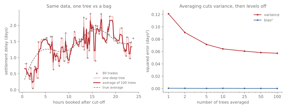
- Bias stays near zero. Averaging deep trees doesn’t make them too simple.
- Variance halves, from 0.121 to 0.057, most of it by the first 10 trees.
- Then it levels off. That’s the floor. From these numbers, the trees’ predictions are correlated at roughly (my estimate: , ignoring the small leftover term).
Honest note: on this small, simple problem, the best single tree from the bias and variance post (depth 2, error 0.154) still beats 100 bagged deep trees (0.180). Bagging removes variance. It doesn’t remove the need to choose a sensible model.
On the settlement-fail data
Now the classification problem from the decision trees post: will this OTC trade fail to settle? Scores are AUC on 5,000 test trades (0.5 is a coin flip, 1.0 is perfect):
| Base tree | One tree | Bag of 200 | Change |
|---|---|---|---|
| Fully grown | 0.584 | 0.743 | big gain |
| Depth 8 | 0.797 | 0.811 | small gain |
| Depth 5 | 0.810 | 0.810 | none |
This table is the whole lesson of bagging:
- It helps a lot when the base model is unstable (high variance), like a fully grown tree.
- It helps little or not at all when the model is already stable. A depth-5 tree changes little between bootstrap samples, so there’s little noise to average away.
And the out-of-bag estimate: from the training data alone, without touching the test set, the bag of fully grown trees reported an AUC of 0.724, close to its real test score of 0.743.
The code
from sklearn.ensemble import BaggingClassifier
from sklearn.tree import DecisionTreeClassifier

bag = BaggingClassifier(
    DecisionTreeClassifier(max_depth=8),   # the model to copy
    n_estimators=200,                       # how many copies
    oob_score=True,                         # test each tree on the rows it never saw
    random_state=0,
)
bag.fit(X_train, y_train)
bag.predict_proba(X_test)[:, 1]             # averaged probability of a fail
bag.oob_score_                              # out-of-bag accuracy estimate
Summary
| Idea | Formula / rule | Remember it as |
|---|---|---|
| Bootstrap | sample rows with replacement | each tree sees a different history |
| Left out | free test data: out-of-bag | |
| Aggregate | average (regression), average or vote (classification) | the committee answer |
| Variance of an average | more models help, until correlation stops them | |
| When it helps | unstable, high-variance models | deep trees: yes; shallow trees: barely |
Next
Random forests: bagging, plus one extra trick that makes the trees less correlated, so the floor drops and averaging works even better.
References
- James, Witten, Hastie, Tibshirani and Taylor, An Introduction to Statistical Learning, with Applications in Python (Springer, 2023), section 8.2.1
- Kevin P. Murphy, Probabilistic Machine Learning: An Introduction (MIT Press, 2022), chapter 18: bagging
- Hastie, Tibshirani and Friedman, The Elements of Statistical Learning (2nd ed., Springer, 2009), chapter 15: the variance of an average of correlated trees (equation 15.1)
- Leo Breiman, “Bagging Predictors”, Machine Learning 24(2), 123–140, 1996
- scikit-learn: bagging meta-estimator