Boosting

Boosting is covered in section 8.2.3 of An Introduction to Statistical Learning, and its classic example is AdaBoost. Boosted trees (the XGBoost and LightGBM family) are among the most common models in banking today for tabular data, so it’s worth understanding what they actually do.

Bagging vs boosting in one picture

In the bias and variance terms: bagging takes complex, unstable models and steadies them. Boosting takes simple, stable models and makes them smarter.

AdaBoost: reweight the mistakes

AdaBoost (adaptive boosting, Freund and Schapire, 1997) was the first widely used boosting method.

1. Give every training example the same weight.
2. Train a weak model, often a stump: a tree with a single question.
3. Measure its weighted error $\risk{\varepsilon}$: the total weight of the examples it got wrong.
4. Give the model a vote $\key{\alpha}$: the lower its error, the bigger its say.
5. Increase the weight of the examples it got wrong, decrease the rest, and repeat from step 2.

The final prediction is a weighted vote of all the models.

The formulas

α, the model's voteε, its errorwrong examplesright examples

The vote of model $t$:

If $\risk{\varepsilon_t} = 0.5$ (a coin flip), $\key{\alpha_t} = 0$: no say. The smaller the error, the larger $\key{\alpha_t}$.

The weight update for each example $i$, depending on whether model $t$ got it wrong or right:

$$w_i \leftarrow w_i \times \begin{cases} \bad{e^{\key{\alpha_t}}} & \bad{\text{if wrong}} \\ \good{e^{-\key{\alpha_t}}} & \good{\text{if right}} \end{cases}$$

Then all the weights are divided by their total, so they add up to 1 again.

Murphy’s Probabilistic Machine Learning: An Introduction (chapter 18, on boosting) writes the same algorithm slightly differently. He calls the vote $\key{\beta_m} = \tfrac{1}{2}\ln\big((1 - \risk{\text{err}_m}) / \risk{\text{err}_m}\big)$, and only multiplies the wrong examples, by $\bad{e^{\key{\alpha_m}}}$ with $\key{\alpha_m} = 2\key{\beta_m}$, before normalising. That’s the same result: either way, a wrong example ends up $e^{2\key{\beta}}$ times heavier than a right one.

Worked example: one round, ten trades

Ten trades, each with weight 0.1. The first stump gets 3 of them wrong:

$$\begin{aligned} \risk{\varepsilon} &= 3 \times 0.1 \\ &= \risk{0.3} \end{aligned}$$ $$\begin{aligned} \key{\alpha} &= \tfrac{1}{2} \ln\!\left(\tfrac{0.7}{\risk{0.3}}\right) \\ &= \key{0.4236} \end{aligned}$$

wrong trades are multiplied by $\bad{e^{\key{0.4236}}} = 1.5275$, right ones by $\good{e^{-\key{0.4236}}} = 0.6547$:

After one round, the 3 wrong trades carry half the total weight (3 × 0.1667 = 0.5), and the 7 right ones the other half. That’s always true after an AdaBoost update: the next model is forced to treat the previous model’s mistakes as half of its whole problem.

A note on scikit-learn’s numbers

scikit-learn’s AdaBoostClassifier (version 1.9) uses the SAMME form of the algorithm. With two classes, the weight it reports is

$$\key{\alpha_t} = \ln\!\left(\frac{1 - \risk{\varepsilon_t}}{\risk{\varepsilon_t}}\right)$$

without the $\tfrac{1}{2}$. That’s exactly Murphy’s $\key{\alpha_m} = 2\key{\beta_m}$. Every vote is twice as big, so the final ranking of predictions is the same; only the printed numbers differ. If you compare a textbook with ada.estimator_weights_, that’s why.

What AdaBoost did on the settlement data

I boosted stumps on the 15,000 made-up OTC trades (5.9% failed). The first three rounds:

Round 1’s error, 0.0589, equals the fail rate. That’s no accident: even trades with a mismatch settle more often than they fail (58% versus 42%), so the first stump says “settles” for everything and gets exactly the fails wrong. Then AdaBoost does its job: the fails now carry half the weight, so round 2’s stump on the same question starts flagging mismatched trades as fails. Round 3 moves on to late booking. Each round fixes a part of what the earlier ones missed.

A single stump scores an AUC of 0.669 on new trades. Boosting 25 of them reaches 0.811.

Gradient boosting: fit the leftover error

Gradient boosting (Friedman, 2001) generalises the idea. Instead of reweighting examples, each new tree is trained to predict what the current model still gets wrong.

For regression with squared error, that’s literally the residuals. An Introduction to Statistical Learning gives it as Algorithm 8.2. Start with $\hat{f}(x) = 0$ and residuals $r_i = y_i$. Then, for each round $b = 1, 2, \dots, B$, fit a small tree $\hat{f}^b$ to the residuals and update:

$$\hat{f}(x) \leftarrow \hat{f}(x) + \lambda \hat{f}^b(x) \qquad \text{(8.10)}$$ $$r_i \leftarrow r_i - \lambda \hat{f}^b(x_i) \qquad \text{(8.11)}$$

The final model is the sum of all the shrunken trees:

$$\hat{f}(x) = \sum_{b=1}^{B} \lambda \hat{f}^b(x) \qquad \text{(8.12)}$$

Plain meaning: start with a rough guess. Look at the errors. Train a small tree to predict the errors. Add a fraction of it to the guess. Repeat. For other losses, like the log loss used for classification, “residuals” become the gradient of the loss, which gives the method its name. The idea is the same.

The learning rate $\lambda$ matters a lot. Each tree only corrects part of the error, so no single tree can push the model too far:

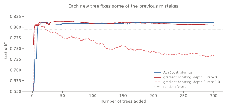
Two lessons from the chart:

• Too high a learning rate overfits fast. At rate 1.0, each tree over-corrects. The score peaks after 9 trees, then falls to 0.734 as the model starts fitting noise.
• Boosting can overfit by adding trees, unlike a random forest. Even at rate 0.1, the score peaks at 44 trees and then slowly declines. In practice you use early stopping: watch a validation score and stop adding trees when it stops improving.

On this data, well-tuned boosting edged out the random forest. That matches common experience on tabular data, but it isn’t a law: with fewer rows or noisier labels, forests often win because they’re harder to overfit.

The code

from sklearn.ensemble import AdaBoostClassifier, GradientBoostingClassifier
from sklearn.tree import DecisionTreeClassifier

ada = AdaBoostClassifier(DecisionTreeClassifier(max_depth=1),   # stumps
                         n_estimators=300, learning_rate=1.0)
ada.fit(X_train, y_train)
ada.estimator_errors_[:3], ada.estimator_weights_[:3]           # epsilon and alpha per round

gb = GradientBoostingClassifier(n_estimators=300, learning_rate=0.1, max_depth=3,
                                validation_fraction=0.1, n_iter_no_change=20)   # early stopping
gb.fit(X_train, y_train)
gb.n_estimators_                                                # trees actually used

For large datasets, scikit-learn’s HistGradientBoostingClassifier, XGBoost and LightGBM are much faster versions of the same idea.

Summary

That completes the ML basics series: what machine learning is, regression versus classification, linear regression, decision trees, bias and variance, bagging, random forests and boosting.

References

• James, Witten, Hastie, Tibshirani and Taylor, An Introduction to Statistical Learning, with Applications in Python (Springer, 2023), section 8.2.3: boosting, Algorithm 8.2 (equations 8.10 to 8.12)
• Kevin P. Murphy, Probabilistic Machine Learning: An Introduction (MIT Press, 2022), chapter 18: AdaBoost (β and α = 2β) and gradient boosting
• Yoav Freund and Robert E. Schapire, “A Decision-Theoretic Generalization of On-Line Learning and an Application to Boosting”, Journal of Computer and System Sciences 55(1), 119–139, 1997
• Jerome H. Friedman, “Greedy Function Approximation: A Gradient Boosting Machine”, The Annals of Statistics 29(5), 1189–1232, 2001
• scikit-learn: AdaBoost and gradient boosting